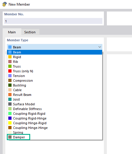
Using the "Damper" member type, you can define a damping coefficient, a spring constant, and a mass. This member type extends the possibilities within the Time History Analysis.
With regard to viscoelasticity, the "Damper" member type is similar to the Kelvin-Voigt model, which consists of the damping element and an elastic spring (both connected in parallel).

For a response spectrum analysis of building models, you can display the sensitivity coefficients for the horizontal directions by story.
These key figures allow you to interpret the sensitivity to stability effects.
- Analysis of time diagrams and accelerograms (acceleration-time diagrams exciting the supports of a structure)
- Combination of user-defined time diagrams with nodal, member, and surface loads, as well as free and generated loads
- Combination of several independent excitation functions
- Linear implicit Newmark analysis or modal analysis in time history
- Structural damping using Raleigh damping coefficients or Lehr's damping value
- Graphical display of results in calculation diagrams
- Result display in individual time steps or as an envelope during the entire time period
- Extensive library of seismic events (accelerograms)
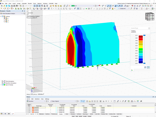
You can display the RWIND results directly in the main program. In the Navigator - Results, select the Wind Simulation Analysis result type from the list above.
Currently, the following results are available, which refer to the RWIND computational mesh:
- Surface pressure
- Surface cp coefficient
- Wall distance y+ (steady flow)
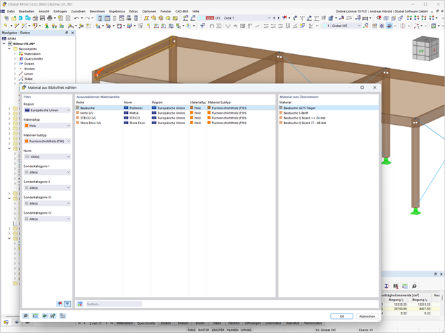
In RFEM and RSTAB, you can design members with the "Laminated Veneer Lumber" material type. The following manufacturers are available:
- Pollmeier (Baubuche)
- Metsä (Kerto LVL)
- STEICO
- Stora Enso
In the ultimate configuration, you can consider strength coefficients for increasing the strengths. The coefficients reducing the strengths are automatically taken into account regardless of this. Try it now!
Go to Explanatory Video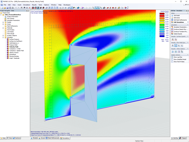
Use RWIND 2 Pro to easily apply a permeability to a surface. All you need is the definition of
- the Darcy coefficient D,
- the inertial coefficient I, and
- the length of the porous medium in the direction of flow L,
to define a pressure boundary condition between the front and back of a porous zone. Due to this setting, you obtain the flow through this zone with a two-part result display on both sides of the zone area.
But that's not all. Furthermore, the generation of a simplified model recognizes permeable zones and takes into account the corresponding openings in the model coating. Can you waive an elaborate geometric modeling of the porous element? Understandable – we have good news for you then! With a pure definition of the permeability parameters, you can avoid complex geometric modeling of the porous element. Use this feature to simulate permeable scaffolding, dust curtains, mesh structures, and so on.
More Information
You have several options available to define masses for a modal analysis. While the masses due to self-weight are considered automatically, you can consider the loads and masses directly in a load case of the modal analysis type. Do you need more options? Select whether to consider full loads as masses, load components in the global Z-direction, or only the load components in the direction of gravity.
The program offers you an additional or alternative option for importing masses: A manual definition of load combinations as of which are the masses considered in the modal analysis. Have you selected a design standard? You can then create a design situation with the Seismic Mass combination type. Thus, the program automatically calculates a mass situation for the modal analysis according to the preferred design standard. In other words: The program creates a load combination on the basis of the preset combination coefficients for the selected standard. This contains the masses used for the modal analysis.
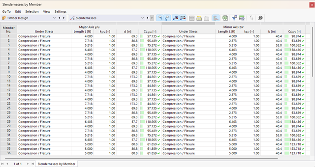
- Stability analyses for flexural buckling, torsional buckling, and flexural-torsional buckling under compression
- Import of the effective lengths from the calculation using the Structure Stability add-on
- Graphical input and check of the defined nodal supports and effective lengths for stability analysis
- Determination of the equivalent member lengths for tapered members
- Consideration of Lateral-Torsional Bracing Position
- Lateral-torsional buckling analysis of the structural components subjected to moment loading
- Depending on the standard, a choice between user-defined input of Mcr, analytical method from the standard, and use of internal eigenvalue solver
- Consideration of a shear panel and a rotational restraint when using the eigenvalue solver
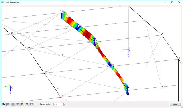
- Graphical display of a mode shape if the eigenvalue solver was used
- Stability analysis of structural components with the combined compression and bending stress, depending on the design standard
- Comprehensible calculation of all necessary coefficients, such as the factors for considering moment distribution or interaction factors
- Alternative consideration of all effects for the stability analysis when determining internal forces in RFEM/RSTAB (second-order analysis, imperfections, stiffness reduction, possibly in combination with the Torsional Warping (7 DOF) add-on)
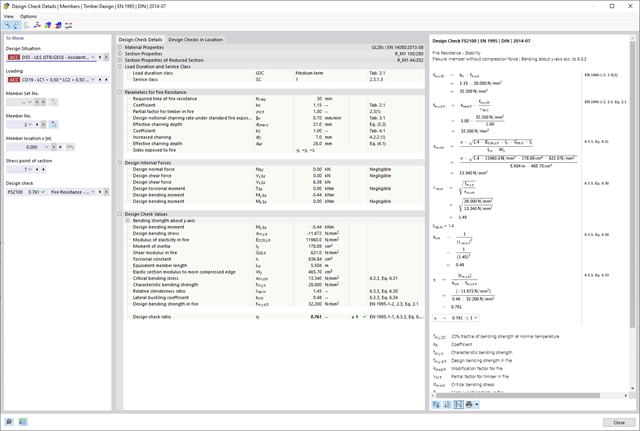
As you probably know, the design checks for the selected members are carried out, taking into account the defined charring time. All necessary reduction factors and coefficients are stored accordingly in the program and are taken into account when determining the load-bearing capacity. That saves you a lot of work.
The effective lengths for the equivalent member design are taken directly from the strength entries. You do not have to enter them again.
After completing the design, the program presents the fire resistance design checks clearly and with all result details. This allows you to follow the results completely transparently. The results also contain all the required parameters, so you can determine the component temperature at the design time.
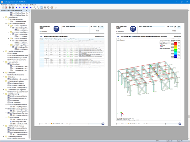
In addition to all these features, the program allows you to integrate all result tables and graphics, including the ultimate and serviceability limit state results,into the global printout report of RFEM/RSTAB as a part of the steel design results.
- Manual specification of critical component temperature or automatic determination of component temperature for desired duration
- A wide range of fire curves: standard temperature-time curve, external fire curve, hydrocarbon curve
- Manual adjustment of the essential coefficients for the determination of the steel temperature
- Consideration of hot-dip galvanizing of structural components for the determination of the steel temperature
- Results of a temperature-time diagram for the gas and steel temperature
- Fire protection cladding as a contour or a box cladding with temperature-independent materials can be considered when determining the temperature
- Design of members made of carbon steel or stainless steel
- Cross-section design checks and stability analyses (equivalent member method) according to EN 1993‑1‑2, Clause 4.2.3
- Design checks of the cross-sections of Class 4 according to EN 1993‑1‑2, Annex E.
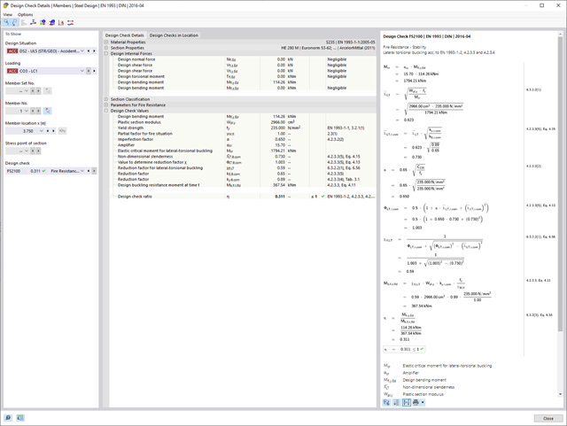
The design checks for the members you have selected are carried out taking into account the governing component temperature. You can perform the cross-section design checks and stability analyses according to EN 1993‑1‑2, Section 4.2.3, in the Steel Design add-on. All reduction factors and coefficients that are necessary are stored accordingly and are taken into account when determining the load-bearing capacity.
The effective lengths for the equivalent member design are taken directly from the strength entries. You don't need to enter them again.
In each design, perform the cross-section classification first. For the cross-sections of Class 4, the design is performed automatically according to EN 1993‑1‑2, Annex E.
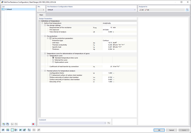
The component temperature to be applied at the design time is determined automatically. You can adjust the coefficients used to determine the temperature. In this step, it is best for you to also select the hot-dip galvanizing. According to the DASt Guideline 027 "Determination of Component Temperature of Hot-Dip Galvanized Steel Components in Case of Fire", a lower emissivity of the steel surface is applied up to a limit temperature. Overall, this gives you a lower temperature for the thus more favorable fire resistance design.

- Calculation of stationary incompressible turbulent wind flow using the SimpleFOAM solver from the OpenFOAM® software package
- Numerical scheme according to the first and second order
- Turbulence models RAS k-ω and RAS k-ε
- Consideration of surface roughness depending on model zones
- Model design via VTP, STL, OBJ, and IFC files
- Operation via bidirectional interface of RFEM or RSTAB for importing model geometries with standard-based wind loads and exporting wind load cases with probe-based printout report tables
- Intuitive model changes via drag & drop and graphical adjustment assistance
- Generation of a shrink-wrap mesh envelope around the model geometry
- Consideration of environmental objects (buildings, terrain, and so on)
- Height-dependent description of the wind load (wind speed and turbulence intensity)
- Automatic meshing depending on a selected depth of detail
- Consideration of layer meshes near the model surfaces
- Parallelized calculation with optimal utilization of all processor cores of a computer
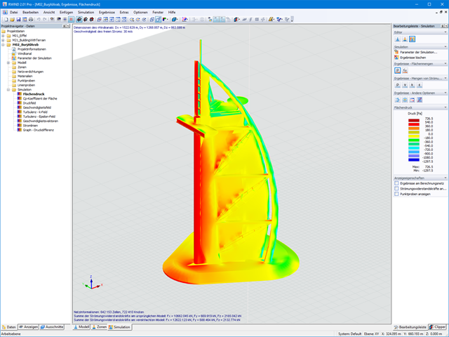
- Graphical output of the surface results on the model surfaces (surface pressure, Cp coefficients)
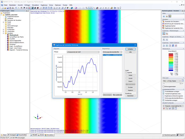
- Graphical output of the flow field and vector results (pressure field, velocity field, turbulence – k-ω field, and turbulence – k-ε field, velocity vectors) on Clipper/Slicer planes
- Display of 3D wind flow via animated streamline graphics
- Definition of point and line probes
- Multilingual user interface (German, English, Czech, Spanish, French, Italian, Polish, Portuguese, Russian, and Chinese)
- Calculations of several models in one batch process
- Generator for creating rotated models to simulate different wind directions
- Optional interruption and continuation of the calculation
- Individual color panel per result graphic
- Display of diagrams with separate output of results on both sides of a surface
- Output of the dimensionless wall distance y+ in the mesh inspector details for the simplified model mesh
- Determination of the shear stress on the model surface from the flow around the model
- Calculation with an alternative convergence criterion (you can select between the residual types pressure or flow resistance in the simulation parameters)
By solving the numerical flow problem, you can obtain the following results on and around the model:
- Pressure on structure surface
- Coefficient Cp distribution on the structure surfaces
- Pressure field about the structure geometry
- Velocity field about the structure geometry
- Turbulence k-ω field about the structure geometry
- Turbulence k-ε field about the structure geometry
- Velocity vectors about the structure geometry
- Streamlines about the structure geometry
- Forces on member-shaped structures that were originally generated from member elements
- Convergence diagram
- Direction and size of the flow resistance of the defined structures
Despite this amount of information, RWIND 2 remains clearly arranged, as is typical for the Dlubal programs. You can specify freely definable zones for a graphic evaluation. Voluminously displayed flow results about the structure geometry are often confusing – you know the problem for sure. That's why RWIND Basic provides freely movable section planes for the separate display of the "solid results" in a plane. For the 3D branched streamline result, you have an option to select between a static and an animated display in the form of moving line segments or particles. This option helps you to represent the wind flow as a dynamic effect.
You can export all results as a picture or, especially for the animated results, as a video.
When starting the analysis in the RFEM or RSTAB application, you trigger a batch process. It places all member, surface, and solid definitions of the model rotated with all relevant coefficients in the numerical wind tunnel of RWIND Basic. Furthermore, it starts the CFD analysis, and returns the resulting surface pressures for a selected time step as FE mesh nodal loads or member loads into the respective load cases of RFEM or RSTAB.
These load cases which contain RWIND Basic loads can then be calculated. Moreover, you can combine them with other loads in load and result combinations.

Compared to the RF‑/DYNAM Pro - Natural Vibrations add-on module (RFEM 5 / RSTAB 8), the following new features have been added to the Modal Analysis add-on for RFEM 6 / RSTAB 9:
- Preset combination coefficients for various standards (EC 8, ASCE, and so on)
- Optional neglect of masses (for example, mass of foundations)
- Methods for determining the number of mode shapes (user-defined, automatic - to reach effective modal mass factors, automatic - to reach the maximum natural frequency)
- Output of modal masses, effective modal masses, modal mass factors, and participation factors
- Masses in mesh points displayed in tables and graphics
- Various scaling options for mode shapes in the Result navigator
The program can also help you here. It determines the bolt forces on the basis of the calculation on the FE model and evaluates them automatically. You can perform the design checks of the bolt resistance for the failure cases tension, shear, hole bearing, and punching shear according to the standard. The program takes care of everything else in this step. It determines all the necessary coefficients and displays them clearly.
- Do you want to perform weld design? The required stresses are also determined on the FE model in that case. Then, the Weld element is modeled as elastic-plastic shell element, where every FE element is checked for its internal forces. (Plasticity criteria is set to reflect failure acc. to AISC J2-4 and J2-5 (weld resistance check) and also J2-2 (base metal capacity check). The design can also be carried out with the partial safety factors according to the selected National Annex.
You can perform the plate design plasticall by comparing the existing plastic strain to the allowable plastic strain. By default this is set to 5% for the AISC 360 but can be specified through user-definition 5% according to EN 1993-1-5, Annex C, or again, user-defined specification.

- Automatic consideration of masses from self-weight
- Direct import of masses from load cases or load combinations
- Optional definition of additional masses (nodal, linear, or surface masses, as well as inertia masses) directly in the load cases
- Optional neglect of masses (for example, mass of foundations)
- Combination of masses in different load cases and load combinations
- Preset combination coefficients for various standards (EC 8, SIA 261, ASCE 7,...)
- Optional import of initial states (for example, to consider prestress and imperfection)
- Structure Modification
- Consideration of failed supports or members/surfaces/solids
- Definition of several modal analyses (for example, to analyze different masses or stiffness modifications)
- Selection of mass matrix type (diagonal matrix, consistent matrix, unit matrix), including user-defined specification of translational and rotational degrees of freedom
- Methods for determining the number of mode shapes (user-defined, automatic - to reach effective modal mass factors, automatic - to reach the maximum natural frequency - only available in RSTAB)
- Determination of mode shapes and masses in nodes or FE mesh points
- Results of eigenvalue, angular frequency, natural frequency, and period
- Output of modal masses, effective modal masses, modal mass factors, and participation factors
- Masses in mesh points displayed in tables and graphics
- Visualization and animation of mode shapes
- Various scaling options for mode shapes
- Documentation of numerical and graphical results in printout report
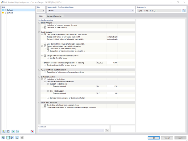
Are you looking for a deformation calculation? Check the Serviceability Configuration, where it can be activated. You can also control the consideration of long-term effects (creep and shrinkage) and tension stiffening between cracks in the dialog box above. The creep coefficient and shrinkage strain are calculated using the specified input parameters, or you can define them individually.
Furthermore, you can specify the deformation limit value individually for each structural component. The max. deformation is defined as the allowable limit value. In addition, you have to specify whether you want to use the undeformed or the deformed system for the design check.
The standards already specify the approximation methods (for example, deformation calculation according to EN 1992‑1‑1, 7.4.3, or ACI 318‑19, 24.3.2.5) that you need for your deformation calculation. In this case, the so-called effective stiffnesses are calculated in the finite elements in accordance with the existing limit state with / without cracks. You can then use these effective stiffnesses to determine the deformations by means of another FEM calculation.
Consider a reinforced concrete cross-section for the calculation of the effective stiffnesses of the finite elements. Based on the internal forces determined for the serviceability limit state in RFEM, you can classify the reinforced concrete cross-section as "cracked" or "uncracked". Do you consider the effect of the concrete between the cracks? In this case, this is done by means of a distribution coefficient (for example, according to EN 1992‑1‑1, Eq. 7.19, or ACI 318‑19, 24.3.2.5). You can assume the material behavior for the concrete to be linear-elastic in the compression and tension zone until reaching the concrete tensile strength. This procedure is sufficiently precise for the serviceability limit state.
When determining the effective stiffnesses, you can take into accout the creep and shrinkage at the "cross-section level." You don't need to consider the influence of shrinkage and creep in statically indeterminate systems in this approximation method (for example, tensile forces from shrinkage strain in systems restrained on all sides are not determined and have to be considered separately). In summary, the deformation calculation is carried out in two steps:
- Calculation of effective stiffnesses of the reinforced concrete cross-section assuming linear-elastic conditions
- Calculation of the deformation using the effective stiffnesses with FEM
- Stability analyses for flexural buckling, torsional buckling, and flexural-torsional buckling under compression
- Import of the effective lengths from the calculation using the Structure Stability add-on
- Graphical input and check of the defined nodal supports and effective lengths for stability analysis
- Lateral-torsional buckling analysis of the structural components subjected to moment loading
- Depending on the standard, a choice between user-defined input of Mcr, analytical method from the standard, and use of internal eigenvalue solver
- Consideration of a shear panel and a rotational restraint when using the eigenvalue solver
- Graphical display of a mode shape if the eigenvalue solver was used
- Stability analysis of structural components with the combined compression and bending stress, depending on the design standard
- Comprehensible calculation of all necessary coefficients, such as the factors for considering moment distribution or interaction factors
- Alternative consideration of all effects for the stability analysis when determining internal forces in RFEM/RSTAB (second-order analysis, imperfections, stiffness reduction, possibly in combination with the Torsional Warping (7 DOF) add-on)

- Stability analyses for flexural buckling, torsional buckling, and flexural-torsional buckling under compression
- Lateral-torsional buckling analysis of the structural components subjected to moment loading
- Import of the effective lengths from the calculation using the Structure Stability add-on
- Graphical input and check of the defined nodal supports and effective lengths for stability analysis
- Depending on the standard, a choice between user-defined input of Mcr, analytical method from the standard, and use of internal eigenvalue solver
- Consideration of a shear panel and a rotational restraint when using the eigenvalue solver
- Graphical display of a mode shape if the eigenvalue solver was used
- Stability analysis of structural components with the combined compression and bending stress, depending on the design standard
- Comprehensible calculation of all necessary coefficients, such as interaction factors
- Alternative consideration of all effects for the stability analysis when determining internal forces in RFEM/RSTAB (second-order analysis, imperfections, stiffness reduction, possibly in combination with the Torsional Warping (7 DOF) add-on)
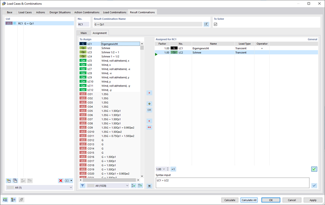
RFEM 6 offers you a wide range of helpful and efficient functions for working with load combinations. You can add the load cases included in load combinations together and then calculate them in consideration of the corresponding factors (partial safety and combination factors, coefficients regarding consequence classes, and so on). Generate the load combinations automatically in compliance with the combination expressions of the standard. You can perform the calculation according to the linear static analysis, second-order analysis, or large deformation analysis, as well as for post-critical analysis. Optionally, you can define whether the internal forces should be related to the deformed or non-deformed structure.
- 3D incompressible wind flow analysis with OpenFOAM® software package
- Direct model import from RFEM or RSTAB including neighboring and terrain models (3DS, IFC, STEP files)
- Model design via STL or VTP files independent of RFEM or RSTAB
- Simple model changes using Drag and Drop and graphical adjustment assistance
- Automatic corrections of the model topology with shrink wrap networks
- Option to add objects from the environment (buildings, terrain ...)
- Wind load determined over the height of the building, depending on standard-specific parameters (velocity, turbulence intensity)
- K-epsilon and K-omega turbulence models
- Automatic mesh generation adjusted to the selected depth of detail
- Parallel calculation with optimal utilization of the capacity of multicore computers
- Results in just minutes for low-resolution simulations (up to 1 million cells)
- Results within a few hours for simulations with medium/high resolution (1‑10 million cells)
- Graphical display of results on the Clipper/Slicer planes (scalar and vector fields)
- Graphical display of streamlines
- Streamline animation (optional video creation)
- Definition of point and line probes
- Display of aerodynamic pressure coefficients
- Graphical display of turbulence properties in the wind field
- Optional meshing using the boundary layer option for the area near the model surface
- Consideration of rough model surfaces possible
- Optional use of a seond-order numerical Order
- Multilingual user interface (for example, German, English, Spanish, French)
- Documentation possible in the RFEM and RSTAB printout report
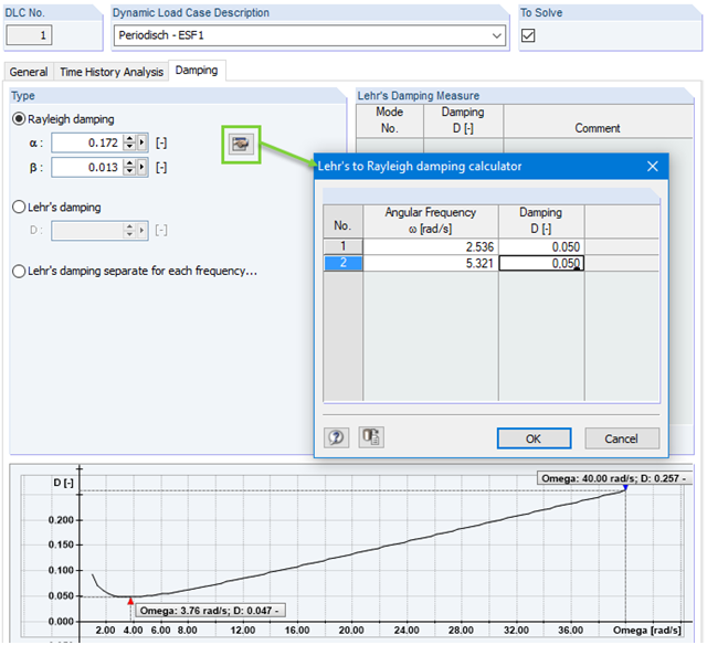
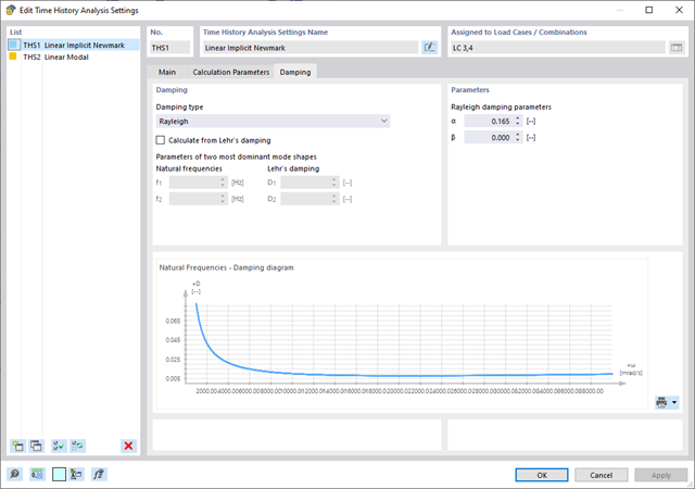
Calculation with consideration of a damping ratio (or Lehr's damping) is not possible in the direct time step integrations. Instead, the Rayleigh damping coefficients must be specified by the user.
In technical literature, the given damping ratio for specific construction forms is, in many cases, only a rough approximation of the real damping ratios. In RF-/DYNAM Pro - Forced Vibrations, it is possible to use the value of the damping ratio to determine the Rayleigh damping. This may occur at one or two natural angular frequencies defined by the user.
.png?mw=640&hash=8cfd0c4bd093c03de543d147ffbf6f5c9250634a)
- User-defined time diagrams as a function of time, in tabular form, or as harmonic loads
- Combination of the time diagrams with RFEM/RSTAB load cases or combinations (enables definition of nodal, member, and surface loads, as well as free and generated loads varying over time)
- Combination of several independent excitation functions
- Nonlinear time history analysis with the implicit Newmark analysis (RFEM only) or the explicit analysis
- Structural damping using Rayleigh damping coefficients or Lehr's damping
- Direct import of initial deformations from a load case or combination (RFEM only)
- Stiffness modifications as initial conditions; for example, axial force effect, deactivated members (RSTAB only)
- Graphical display of results in a time history diagram
- Export of results in user-defined time steps or as an envelope
When performing the design of tension, compression, bending, and shear loading, the module compares the design values of the maximum load capacity to the design values of the actions.
If the components are subjected to both bending and compression, the program performs an interaction. In RF-/STEEL EC3, you can determine the factors according to Method 1 (Annex A) or Method 2 (Annex B).
The flexural buckling design requires neither the slenderness nor the elastic critical buckling load of the governing buckling case. The module automatically calculates all required factors for the bending stress design value. RF-/STEEL EC3 determines the elastic critical moment for lateral-torsional buckling for each member on every x-location of the cross-section. If required, you only need to specify lateral intermediate supports of the individual members/sets of members, definable in one of the input windows.
If members are selected for the fire resistance design in RF-/STEEL EC3, there is another input window available where you can enter additional parameters, such as: a coating or cladding type. Global settings cover the required time of fire resistance, temperature curve, and other coefficients. The printout report lists all intermediate results and the final result of the fire resistance design. Furthermore, it is possible to print the temperature curve in the report.
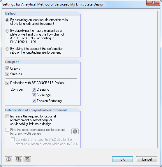
The deformation analysis according to the approximation method defined in standards (for example, deformation analysis according to EN 1992‑1‑1, 7.4.3) applies to the calculation of "effective stiffnesses" in the finite elements in accordance with the existing limit state of the concrete with or without cracks. These stiffnesses are used to determine the surface deformation by repeated FEM calculation.
The effective stiffness calculation of finite elements takes into account a reinforced concrete cross-section. Based on the internal forces determined for the serviceability limit state in RFEM, the program classifies the reinforced concrete cross-section as 'cracked' or 'uncracked'. If the tension stiffening at a section should be considered as well, a distribution coefficient (according to EN 1992-1-1, Eq. 7.19, for example) is used. The material behavior for the concrete is assumed to be linear-elastic in the compression and tension zone until the concrete tensile strength is reached. This is reached exactly in the serviceability limit state.
When determining the effective stiffnesses, creep and shrinkage are taken into account at the "cross-section level". The influence of shrinkage and creep in statically indeterminate systems is not taken into account in this approximation method (for example, tensile forces from shrinkage strain in systems restrained on all sides are not determined and must be considered separately). In summary, RF-CONCRETE Deflect calculates deformations in two steps:
- Calculation of effective stiffnesses of the reinforced concrete cross-section assuming linear-elastic conditions
- Calculation of the deformation using the effective stiffnesses with FEM
- Automatic consideration of masses from self-weight
- Direct import of masses from load cases or load combinations
- Optional definition of additional masses (nodal, linear, surface masses, as well as inertia masses)
- Combination of masses in different mass cases and mass combinations
- Preset combination coefficients according to EC 8
- Optional import of normal force distributions (in order to consider prestress, for example)
- Stiffness modification (for example, deactivated members or stiffnesses can be imported from RF-/CONCRETE)
- Consideration of failed supports or members
- Definition of several natural vibration cases (for example, to analyze different masses or stiffness modifications)
- Results of eigenvalue, angular frequency, natural frequency, and period
- Determination of mode shapes and masses in nodes or FE mesh points
- Results of modal masses, effective modal masses, and modal mass factors
- Visualization and animation of mode shapes
- Various scaling options for mode shapes
- Documentation of numerical and graphical results in the printout report
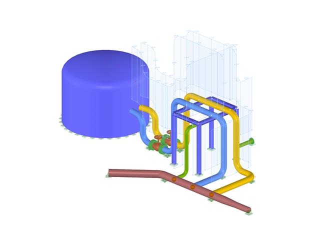
- Graphical input of piping systems and piping components
- Illustrative visualization of piping systems and piping components in RFEM graphic window
- Comprehensive libraries for piping cross‑sections and materials
- Comprehensive libraries for flanges, reducers, tees, and expansion joints
- Consideration of piping structure (insulation, lining, tin‑plate)
- Automatic calculation of stress intensification factors and flexibility factors
- Specific piping action categories for load cases
- Optional automatic combinatorics of load cases
- Consideration of material properties (modulus of elasticity, coefficient of thermal expansion) either during operating temperature (default setting) or during reference (assembly) temperature of material
- Consideration of strain and uplift due to pressure (Bourdon effect)
- Interaction between the supporting structure and the piping system